Master The Art Of Conditional Formatting In Excel 2024

Imagine you have just finished creating a masterpiece of a spreadsheet in Excel, consisting of data, numbers, and information. Now imagine if there’s a way to not only make the spreadsheet informative but visually appealing and organized as well. Well, conditional formatting in Excel is the feature that allows you to do just that.

Conditional formatting in Excel not only helps you make your spreadsheet visually appealing but also helps you effortlessly highlight and bring attention to specific aspects of your data in real-time in your spreadsheet.

In this digital era of cells, rows, and numbers, conditional formatting in Excel is your secret weapon to transform your boring spreadsheet into visually appealing, organized, and easy-to-read.

Let’s unleash the power of visual clarity in Excel while learning conditional formatting in Excel.

Conditional Formatting in Excel

Conditional Formatting in Excel is a way to make your data easy to read and understand by highlighting certain values in the spreadsheet. Conditional formatting uses criteria or you can also say conditions and rules according to which it changes the appearance of a selected cell range in the spreadsheet bringing attention to the specific aspects of your data. 

In simple language, conditional formatting is a feature in Excel that lets you format the background of a cell and text style based on certain conditions or criteria highlighting values that meet the desired condition.

Why Use Conditional Formatting in Excel?

Conditional formatting in Excel helps you highlight certain values based on the criteria that meet certain conditions. This allows you to quickly read, and identify specific data in the spreadsheet that you are looking for in real time.

Conditional formatting not only helps you save time while reading data on a spreadsheet but it also helps you organize your spreadsheet making it more informative and easy to read.

How to Access Conditional Formatting in Excel?

Conditional formatting is a feature available in Excel that is easy to access. Here’s how you can access conditional formatting in Excel. For this tutorial, I’ll not only teach you how you can access this feature but I’ll also try to teach and show you how to use conditional formatting in Excel using certain conditions. I’ll show you how you can use conditional formatting to find out in how many subjects a student failed and scored below 35 marks.

Tutorial For Accessing Conditional Formatting in Excel: Highlight Cells Rules

Using “Less Than” in Conditional Formatting

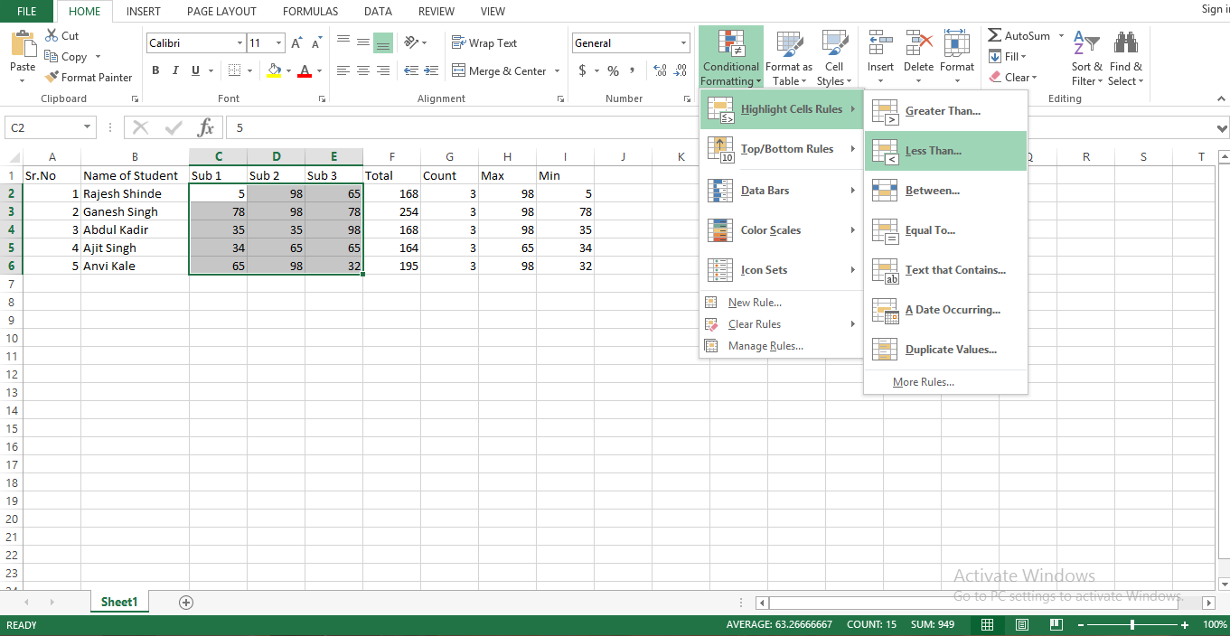
Select the desired range that you want to create rules or conditions for. As you can see in the below screenshot, I have selected a range of subjects as I’ll be going to use a condition to find out how many subjects a student failed in and scored below 35 marks.

• After selecting the range click on the Home tab, go to Conditional formatting, then select the condition less than.

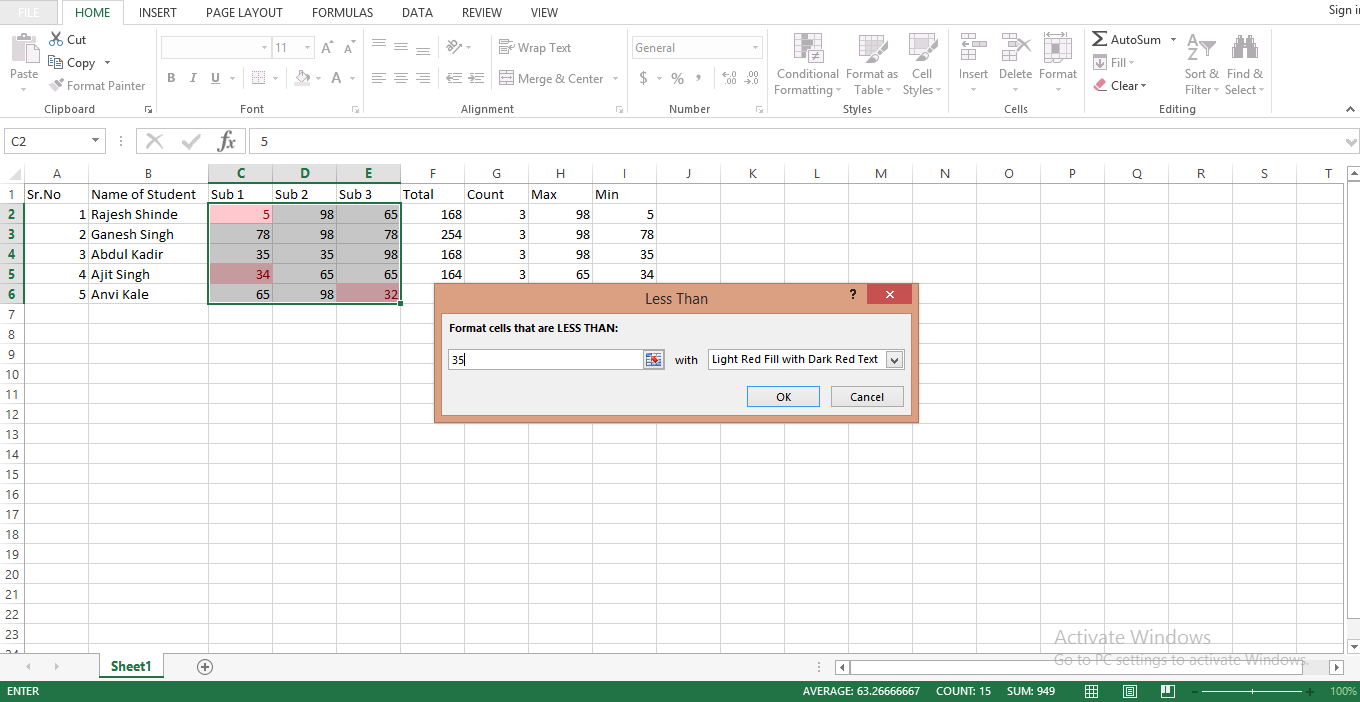
• A dialog box will appear after you click on Less than. Enter the value that you want to identify and highlight in your spreadsheet. In this case, we are looking to identify the number of subjects a student scored below 35 marks. Simply put the value 35 in the dialog box with the formatting style Light Red Fill with Dark Red Text and Viola! You are done.

• You can see the number of subjects a student scored below 35 marks is now highlighted in the spreadsheet.

Note- You may also use custom format as per your need and requirement to highlight the specific aspect of your spreadsheet.

Using “Greater Than” in Conditional Formatting In Excel

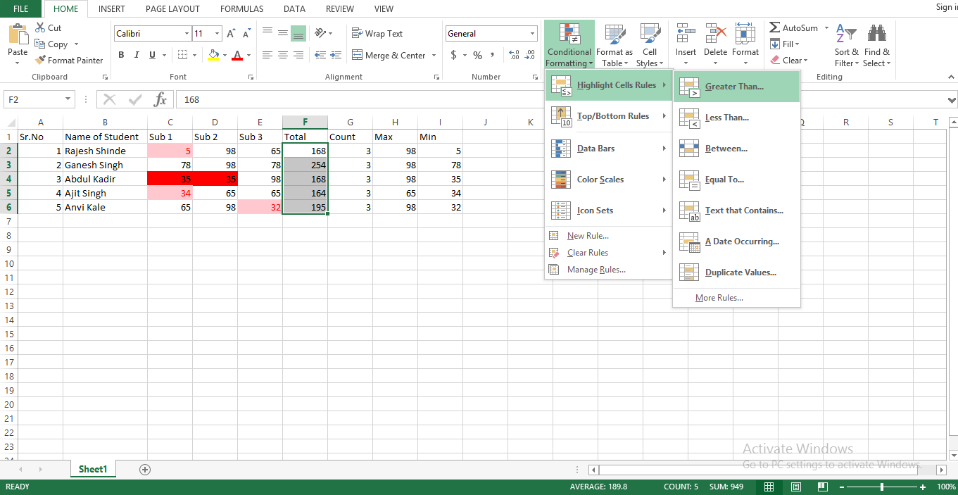
You can use the same method for different ranges to highlight specific aspects of your spreadsheet. For example, if you want to highlight how many students scored more than 200 in total, you can use conditional formatting to highlight the values that meet the conditions.

• Use the screenshot given below for a better understanding. This time we are using the condition Greater Than as we need to identify the number of students who scored more than 200 marks in total.

• After selecting the range simply go to the Home tab> Conditional formatting> Greater Than.

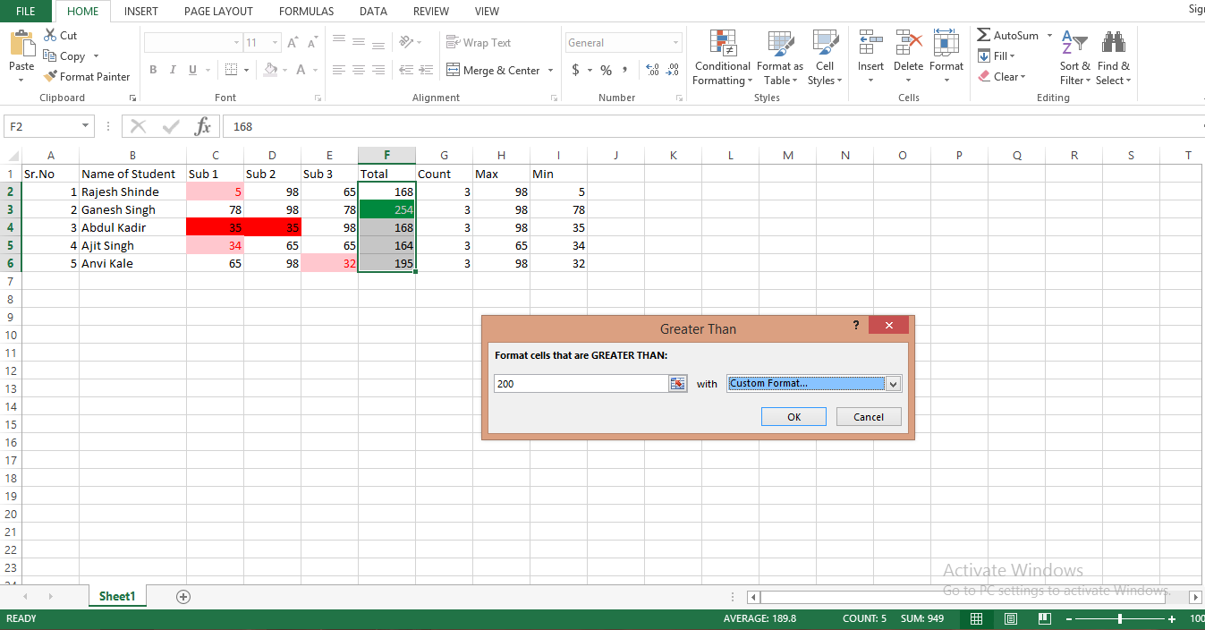
• A dialog box will appear, enter the value 200 with the formatting style custom. I have used green color to highlight the value that meets our condition.

• As you can see Ganesh Singh is the only student who scored more than 200 marks in total.

Using “Clear Rules” in Conditional Formatting

Now, if you made any error in the values or while selecting the range and need to clear rules or conditions from your spreadsheet you can do that too.

• Simply select the range you want to clear the rule from.
• Go to conditional formatting.
• Scroll down to Clear Rules.
• Next, it will ask you to choose whether you want to clear the rule from selected cells or from the entire sheet.
• Choose the option Clear Rules from the selected cell as we just want to clear rules from our selected range.

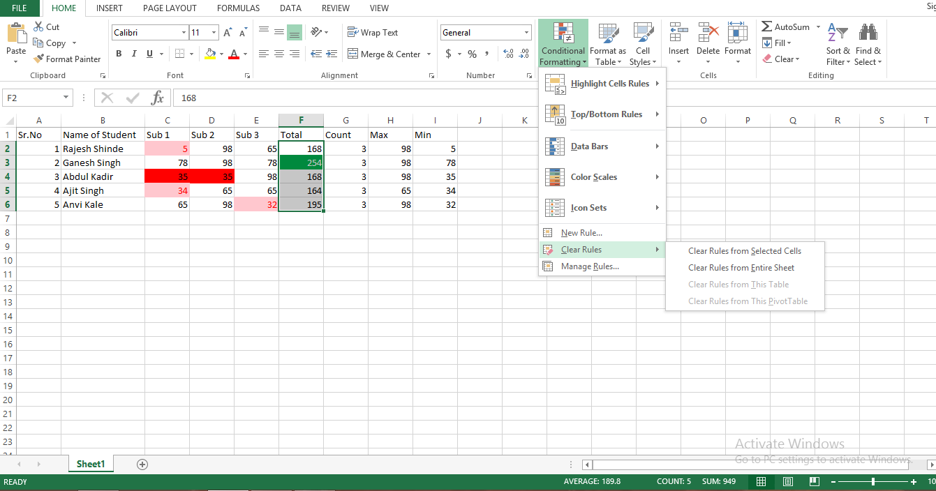
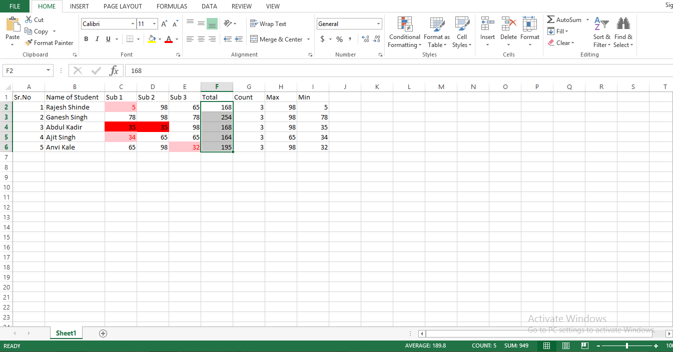
• As you can see the condition from our selected cells has now been cleared.

Understanding Different Conditions in Conditional Formatting In Excel

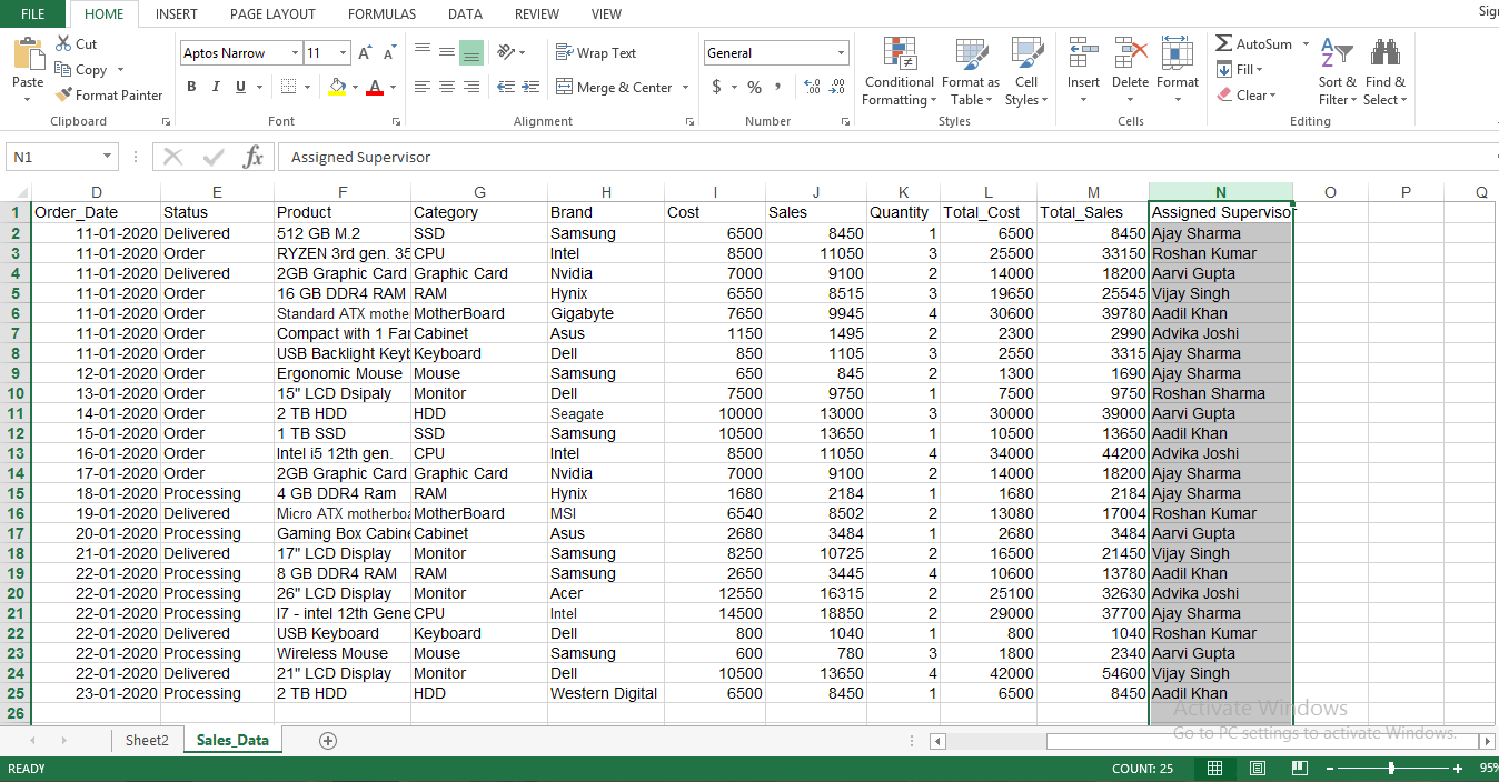
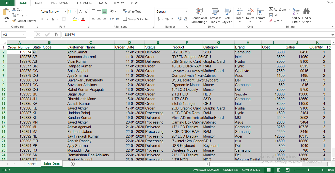
Now, let’s try conditional formatting in Sales data to deeply understand the core principle and uses of conditional formatting in Excel.

For this tutorial, I’ll be using another demo data sheet to teach you some of the important features of conditional formatting. For this tutorial, we will be focusing on highlighting the number of assigned supervisors with the same name. For example, we will be looking for the number of assigned supervisors with the name Ajay Sharma.

Using “Equal To” in Conditional Formatting

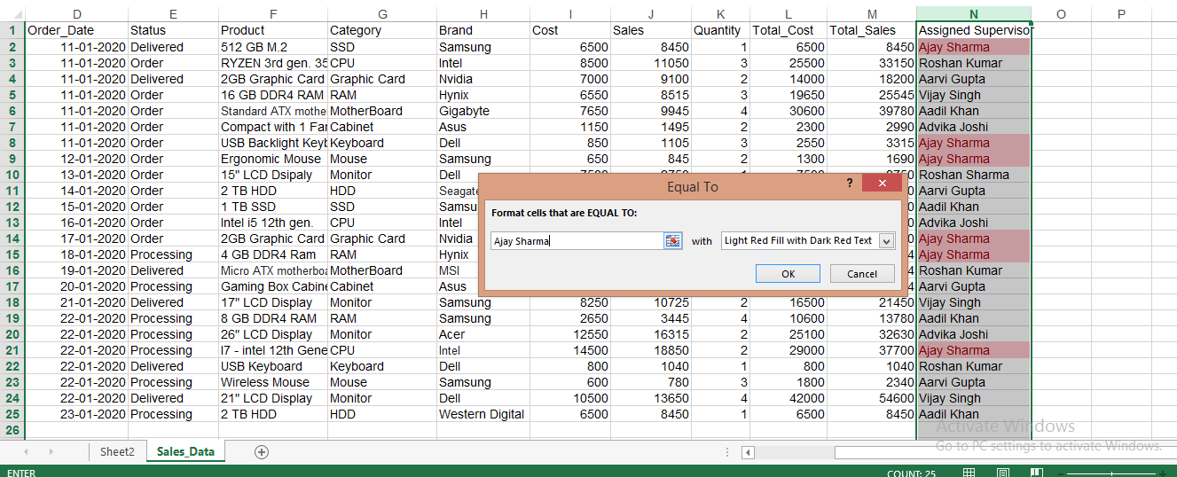
The first thing we need to do is to select the range. In our case, we need to identify and highlight the number of assigned supervisors with the name Ajay Sharma. We will select the range of Assigned Supervisors( N)

• Now go to conditional formatting> Highlight Cell Rules and then click on Equal To. Equal to condition is used to highlight the value with the exact equal or same value.

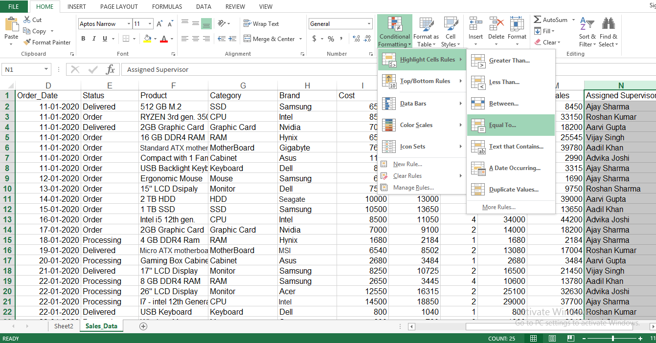
• A dialog box will appear after you click on Equal To. Enter the value you need to highlight in the dialog box (Ajay Sharma) with the default formatting style of Light Red Fill with Dark Red Text and click on OK. You can always customize the formatting style as per your needs.
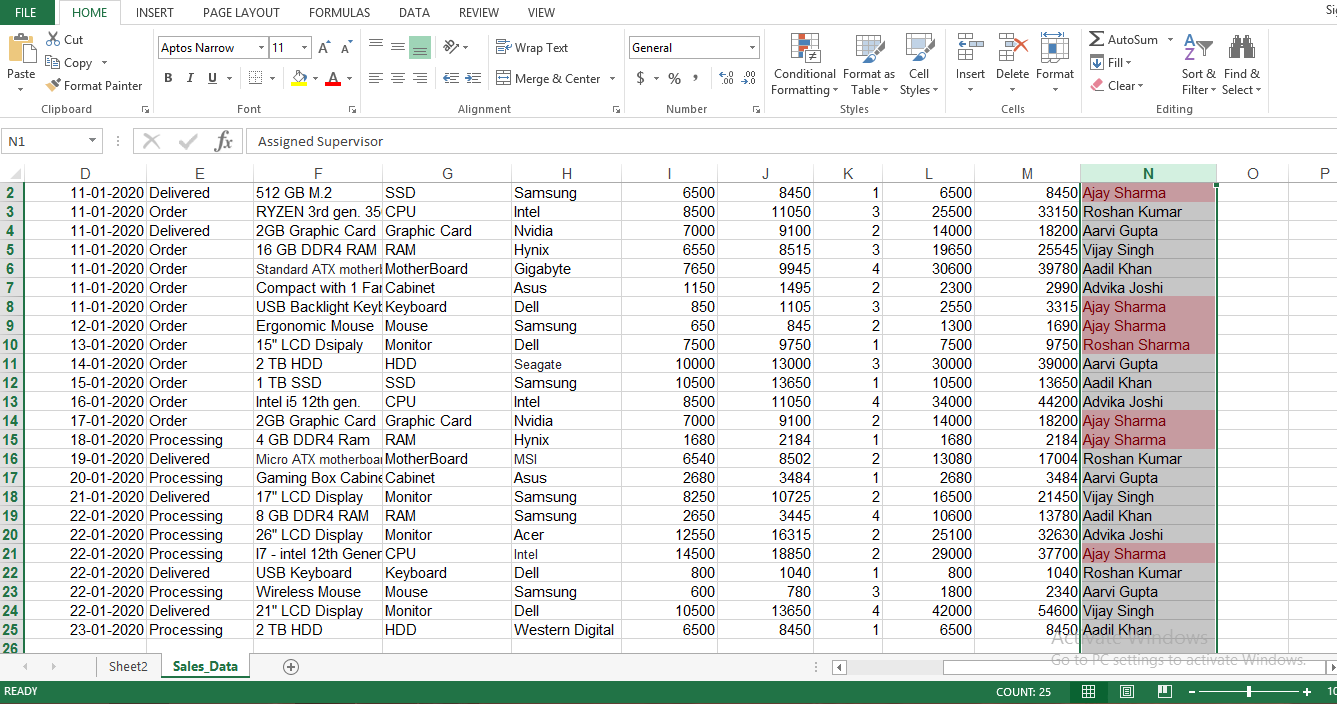
• As you can see all the assigned supervisors with the name Ajay Sharma are now being highlighted in the data.

Using “Text That Contains” in Conditional Formatting

Let’s take another example to understand another feature for using conditional formatting in Excel. Suppose, you want to identify the number of people working in your company with the surname Sharma among assigned supervisors.

• Select the range which is again going to be the column N Assigned Supervisors.
• Go to conditional formatting, and select the “Text That Contains” option from the menu.

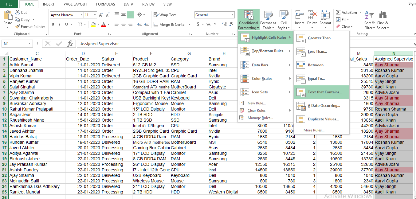
• After you click on the Text That Contains option, a dialog box will appear. In the dialog box enter the value you want to highlight and click OK. In this case, we want to highlight all the people with the surname Sharma among assigned supervisors.

• Now as you can see all the workers with the surname Sharma among assigned supervisors are now being highlighted.

Note: In conditional formatting option “Equal To” allows you to highlight and identify the exact value that you enter in the appeared dialog box whereas option “Text That Contains” allows you to highlight the values that could be different but at the same time also contain the text that you input in the appeared dialog box. For reference and better understanding review the screenshots mentioned above.

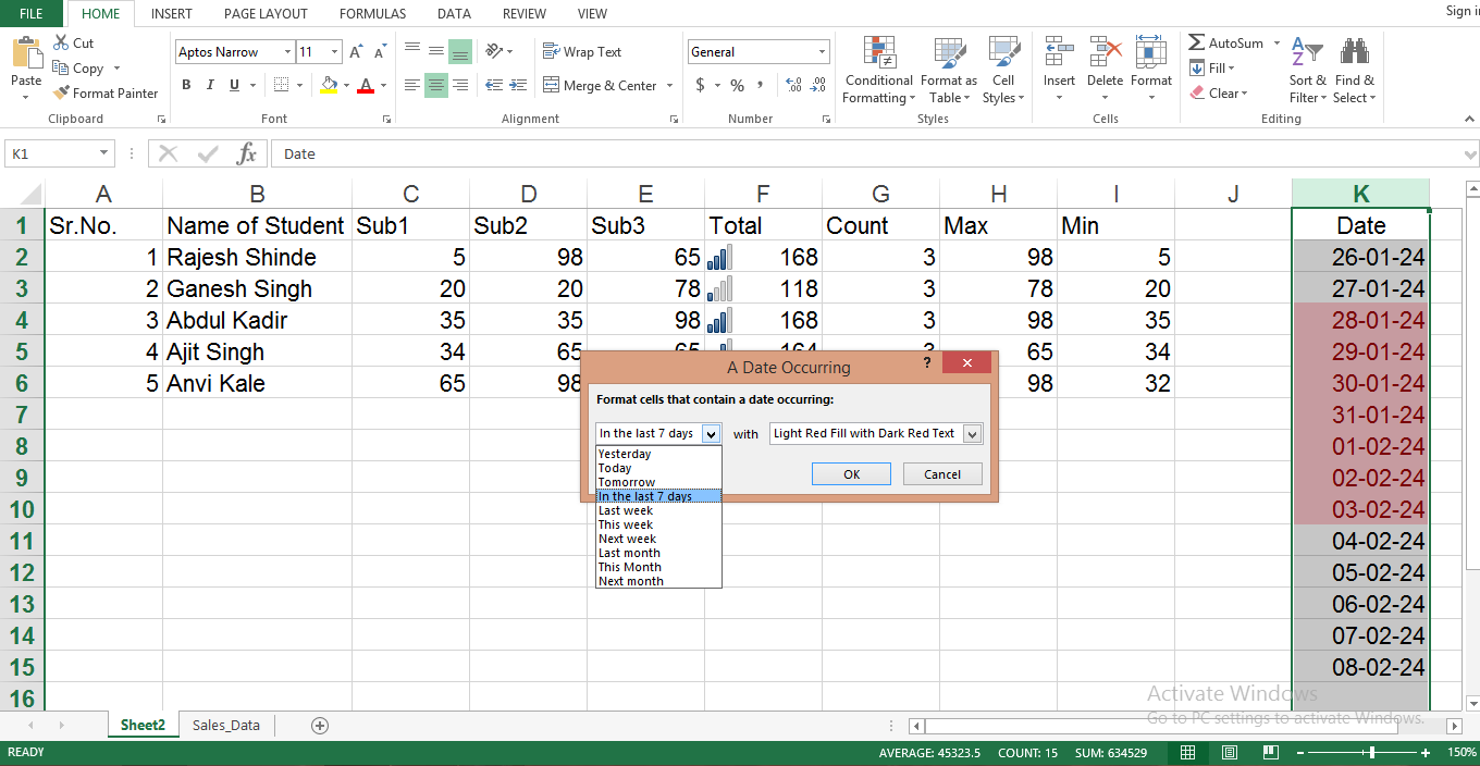
Using A Date Occurring in Conditional Formatting

Let’s get into the next feature in conditional formatting in Excel which is A Date Occurring.

• Select the range then go to Conditional formatting> Highlight Cells Rules> then select the option “A Date Occurring“.

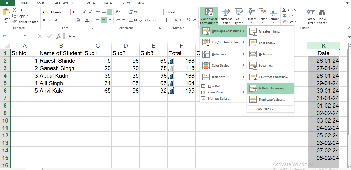
• “A Date Occurring” feature is majorly used in sales to highlight the sales on a particular date or within a particular period of time.
• You may use this feature to track sales and orders from today’s date to next month.

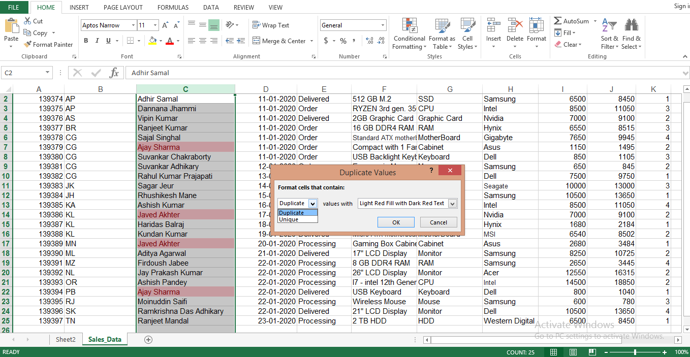
Using Duplicate Values in Conditional Formatting

Let’s take a look at another feature in conditions formatting which is “Duplicate Values“. “Duplicate values” is the feature that allows you to highlight the duplicate or repetitive values in your data.

Let’s understand it with an example. Suppose you have a customer list or a list and you want to highlight the names of your repetitive customers. You can do that using Duplicate values in conditional formatting.

• Select range then go to Conditional formatting> Highlight Cells Rules and select Duplicate Values.

• A dialog box will appear after you click on Duplicate Values. Select the option Duplicate and click on OK.
• As you can see all the repetitive values are now highlighted in the spreadsheet.

Tutorial For Accessing Conditional Formatting in Excel: Top/Bottom Rules

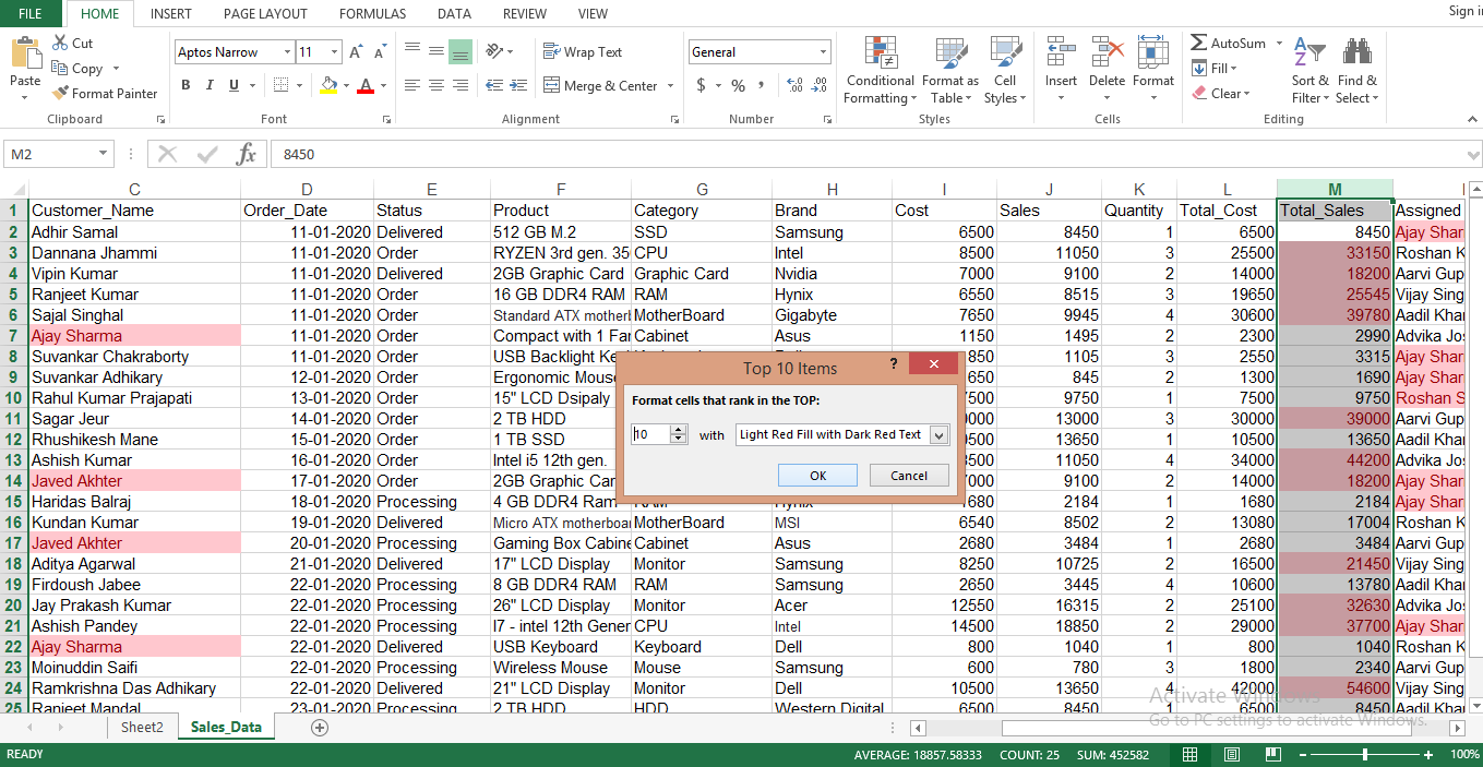
Using Top 10 Items in Conditional Formatting

The feature Top 10 Items is used to highlight the top 10 values of specific aspects of your spreadsheet. For example, if you want to highlight the top 10 sales in your data you can do that using this feature in the top/bottom rules.

• Select a range then go to conditional formatting then click no Top/Bottom Rules and select the option Top 10 Items from the menu.

• After you click on the Top 10 Items, a dialog box will appear where you can select the number of top values you want to highlight within the selected range.
• You can use this feature to highlight the top 10 to top 3 to top 50. It basically depends on you on how much data you want to highlight and look into.

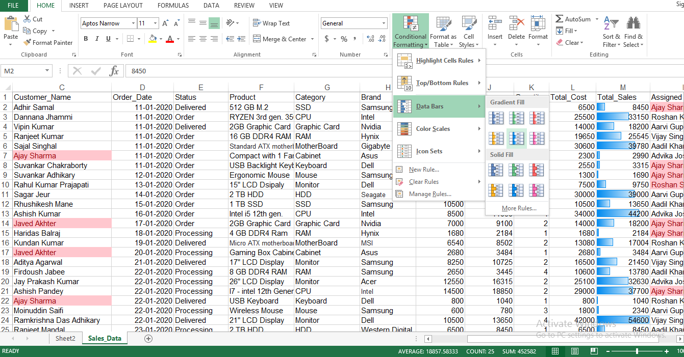
Using “Data Bars” in Conditional Formatting

“Data bars” is a feature in conditional formatting that allows you to make your data visually appealing and easy to read by adding graphical representation to your spreadsheet.

• To access Data Bars go to conditional formatting, select Data Bars from the from-down menu, and choose the style you want to add to your data.
• In the screenshot, I have used Gradient Fill for the formatting style. Complete fill of bars represents the highest values whereas no fill or less fill represents the lowest value.
• This feature is used to add a graphical representation to your data to make it easy to read and visually appealing.

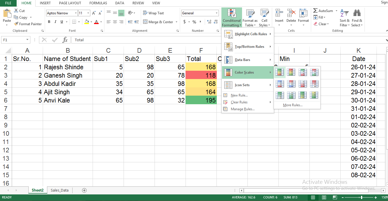
Using “Color Scale” in Conditional Formatting

The “Color scale feature” is quite the same as of “Data Bars” but the only difference between both features is that data Bars are used to highlight the highest to lowest values in the data whereas the Color Scale feature is used to highlight data within the same range using different colors.

• To access the Color Scale feature you need to select a range, then go to conditional formatting and scroll down to the option Color Scale.
• Here you can see the different Color Scale styles, you may choose any color combination you want for your data from the menu and then click ok.
• As you can see values between 164 to 168 have been highlighted with yellow color as they fall in the same range whereas numbers 195 and 118 have been highlighted with green and red color respectively as 195 is the highest and 118 is the lowest.

Using “Icon Sets” in Conditional Formatting

“The Icon Sets” is another interesting feature in conditional formatting that allows you to highlight a selected range of data with unique icons.

• Select range then go to conditional formatting and scroll down to the Icon sets option.
• In the Icon Sets option, you will find different types of icons that you can choose to highlight a selected range of data in your spreadsheet. For example, Directional, Shapes, Indicators, and Ratings.

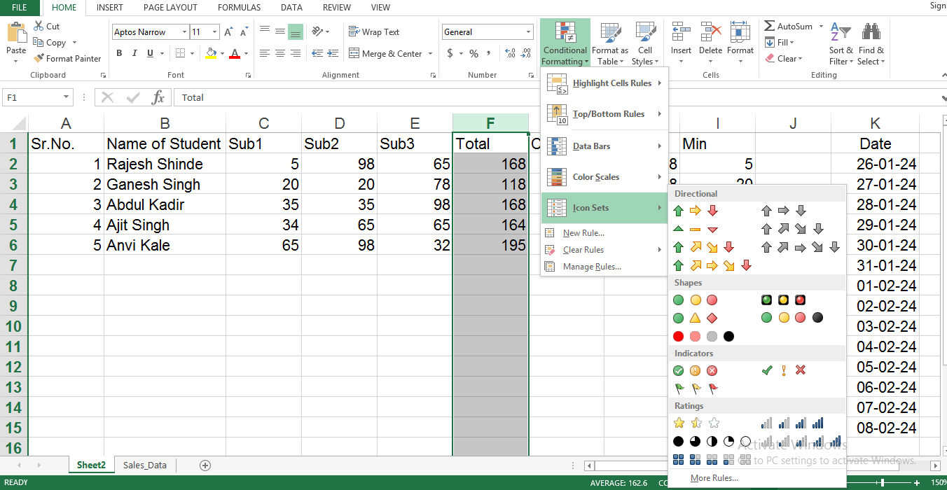
• Icon Sets give you different icons for different values for the selected range of data.

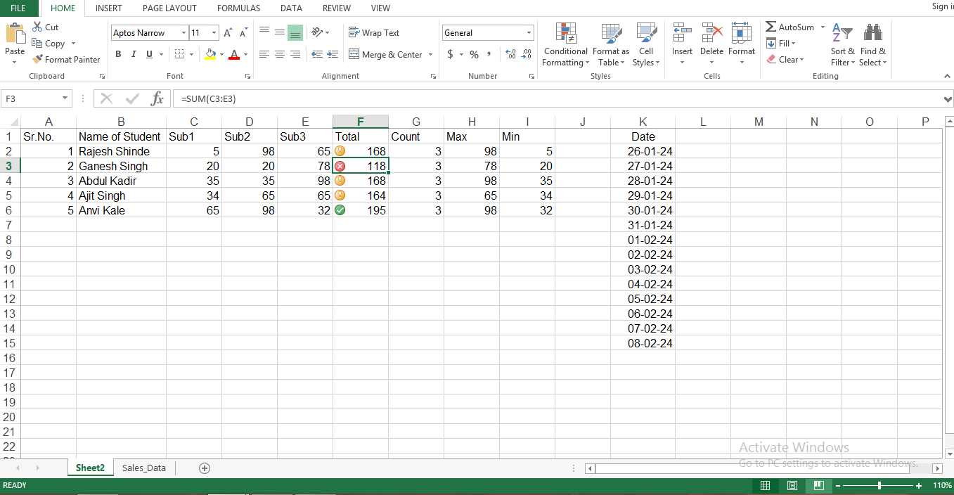
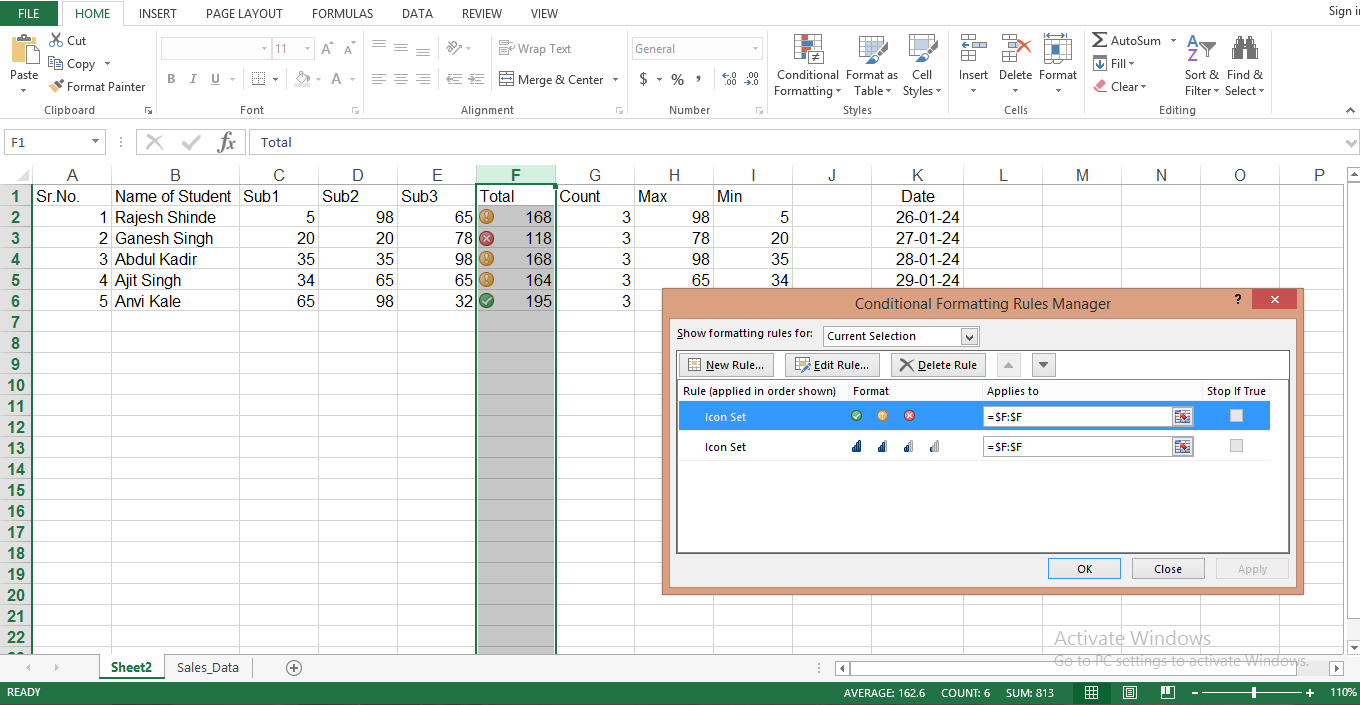
How to Manage Rules for Icon Sets in Conditional Formatting?

Manage Rules is the option available in the conditional formatting that allows you to manage rules for each icon in the Icon sets option.

• To access manage rules for Icon Sets, select the range the Icon sets formatting is already applied.
• Go to conditional formatting and scroll down to the last option Manage Rules.

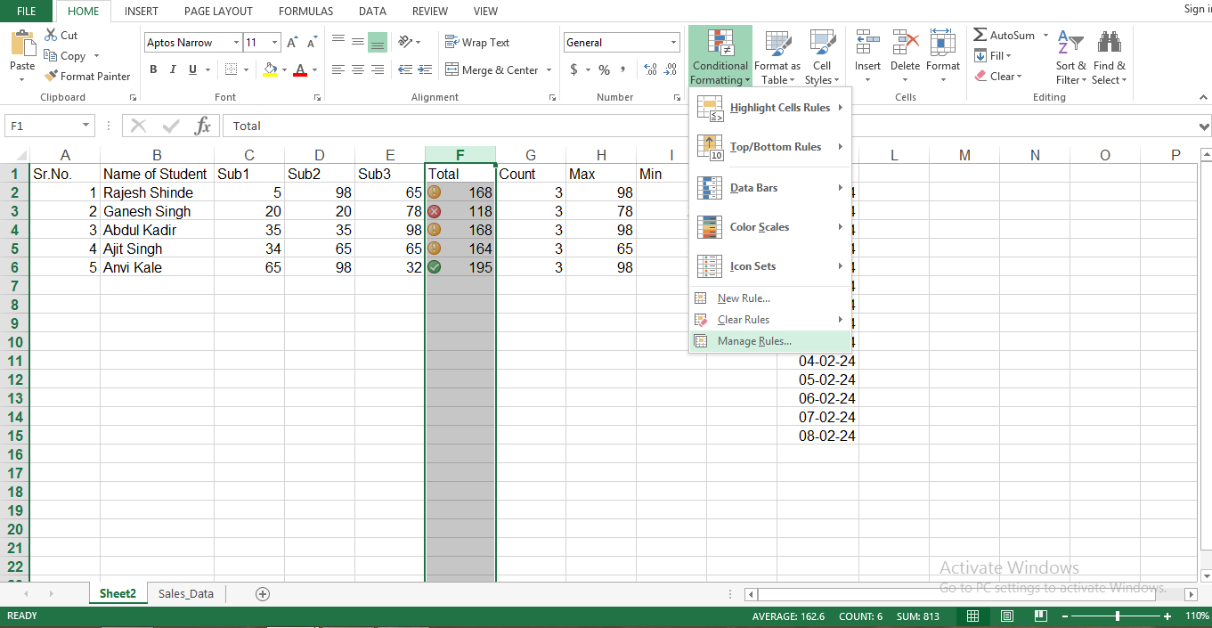
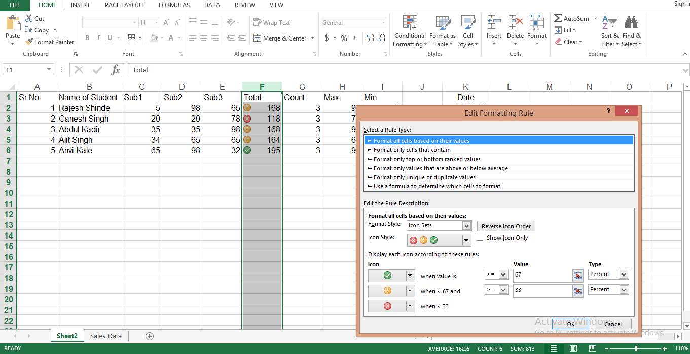
• Now select the Icons Set you want to edit or manage the rules for from the popup window and click on the Edit Rule button in the popup window.

• A new window will pop up after you click on the Edit Rule button. In this new window, you will find various options. In this new window, you can edit the format style and icon style and even display each icon according to the rules you set.
• This is how you can assign conditional formatting in your spreadsheet using these features.

Tutorial For Accessing Advanced Conditional Formatting in Excel

Let’s now dive into the advanced features of conditional formatting in Excel. For this tutorial, we will be highlighting the complete details of the delivered status in our demo spreadsheet.

• First, we need to select the range of the data that we want to apply the rule to highlight the values that meet the condition of our rule.
• To select the range we need to click on row 2 then CTRL + SHIFT + arrow down.

After selecting the range, go to conditional formatting and scroll down to the option New Rule.

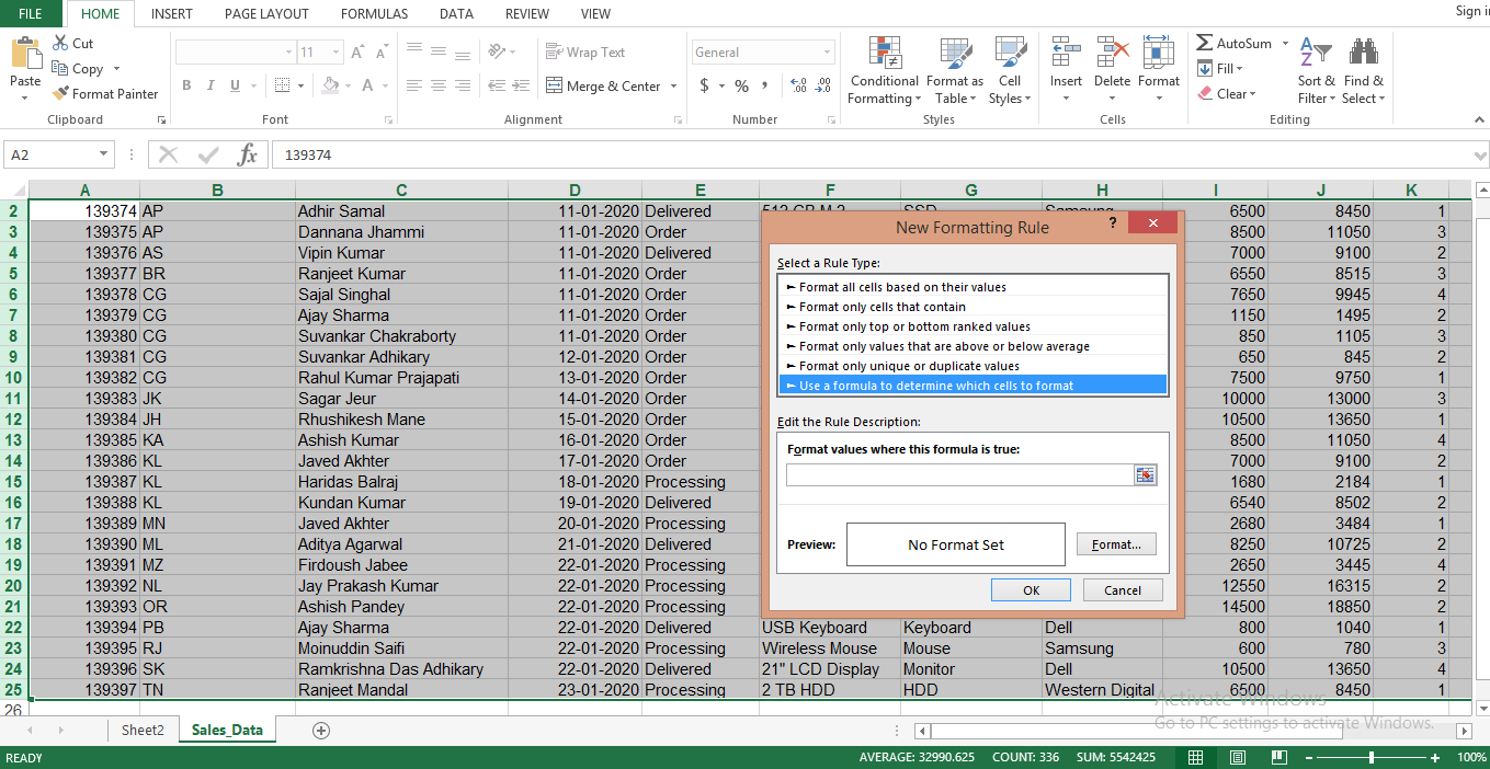
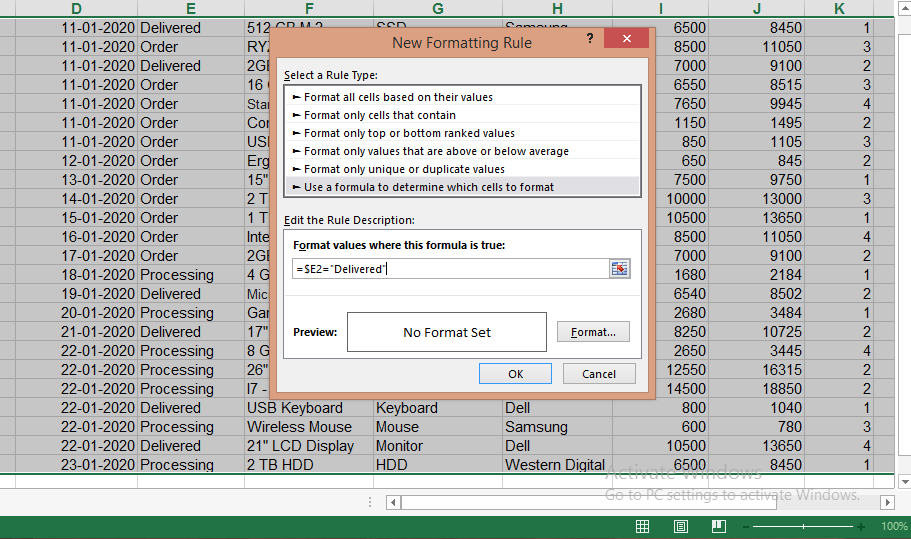
• Click on the New Rule option and a new dialog box will appear on your screen.

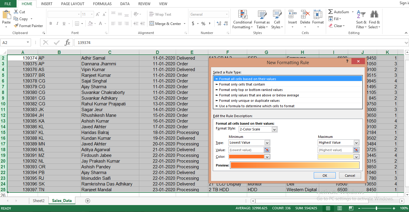
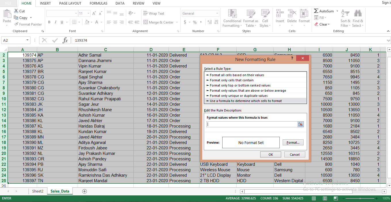
• Now click on the option “Use a formula to determine which cells to format.”

Now take down your cursor and click on the empty place under the text Format Values Where This Formula is True.

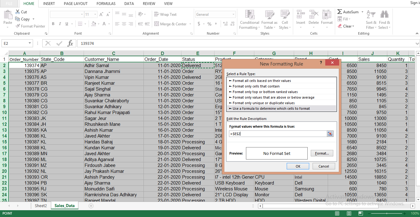
• Now go to row 2 and click on the text Delivered under status in column E.
• Now you can see the value has been added inside the popup window which is” =$E$2”

• $ sign is used to fix or lock a specific row, column, and cell in your spreadsheet and that is why we need to remove it before 2. This way we will be able to collect and highlight all the data on the delivered status for every row.
• We are not removing the $ sign from E because the E column is the only column that has the data on the delivered status.

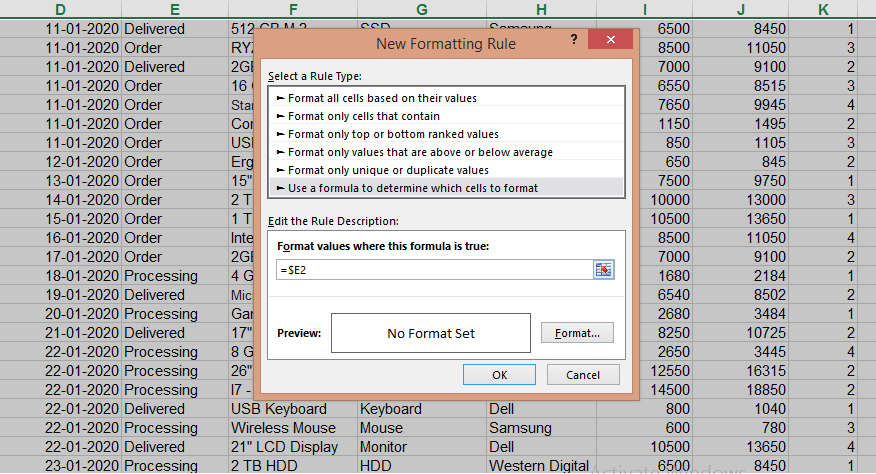
• Now to highlight all the delivered statuses we need to put in a formula that is =$E2=”Delivered”.
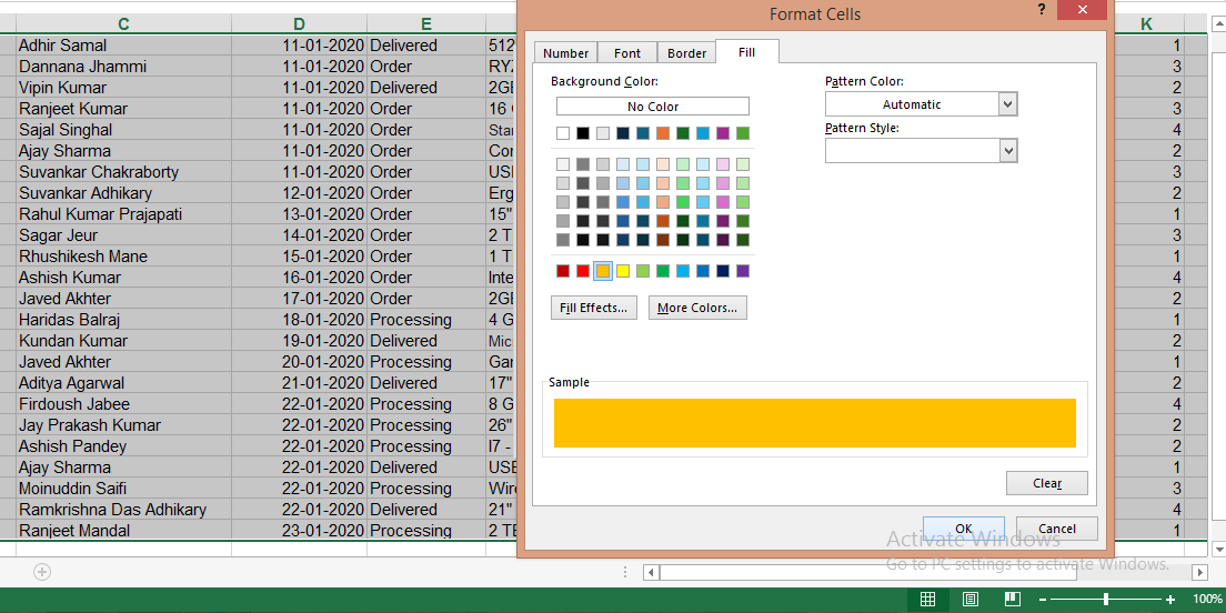
• After putting the formula click on the format button.

• A new dialog box will appear after you click on the format button.

• Now click on the fill button, select the color you want to use to highlight the data in your spreadsheet, and click on the ok button.

• A new window will pop up just click on the ok button.

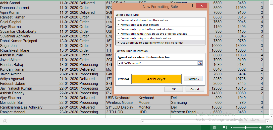
• As you may see all the delivered statuses are now highlighted and you can easily read the data in your spreadsheet.

Note: This method can be used for any row and any column, all you need to do is remember the process and the correct way to create a rule.

Bottom Line

Congratulations! You have now mastered the art of turning your boring spreadsheet into colorful and informative masterpieces. Now that you have learned conditional formatting in Excel you can now go and dress up your data, rows, and cells in style.

I have tried to cover almost all the features from basics to advanced in this tutorial post for conditional formatting in Excel. I hope you find this tutorial useful and keep learning more about all the interesting things that you can do while utilizing the skills you are learning online.